
Modeling of Diurnal Changing Patterns in Airborne Crop Remote Sensing Images
by
Dongdong Ma
1, 
Tanzeel U. Rehman
1,
Libo Zhang
1,
Hideki Maki
2,
Mitchell R. Tuinstra
3 and
Jian Jin
1,* 1
Department of Agricultural and Biological Engineering, Purdue University, West Lafayette, IN 47907, USA
2
Health and Crop Sciences Research Laboratory, Sumitomo Chemical Co., Ltd., Hyogo 665-8555, Japan
3
Department of Agronomy, Purdue University, West Lafayette, IN 47907, USA
*
Author to whom correspondence should be addressed.
Remote Sens. 2021, 13(9), 1719; https://doi.org/10.3390/rs13091719
Submission received: 29 March 2021
/
Revised: 26 April 2021
/
Accepted: 26 April 2021
/
Published: 29 April 2021
(This article belongs to the Special Issue Precision Agriculture Using Hyperspectral Images)
Abstract
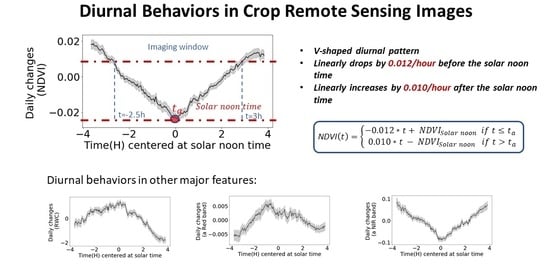
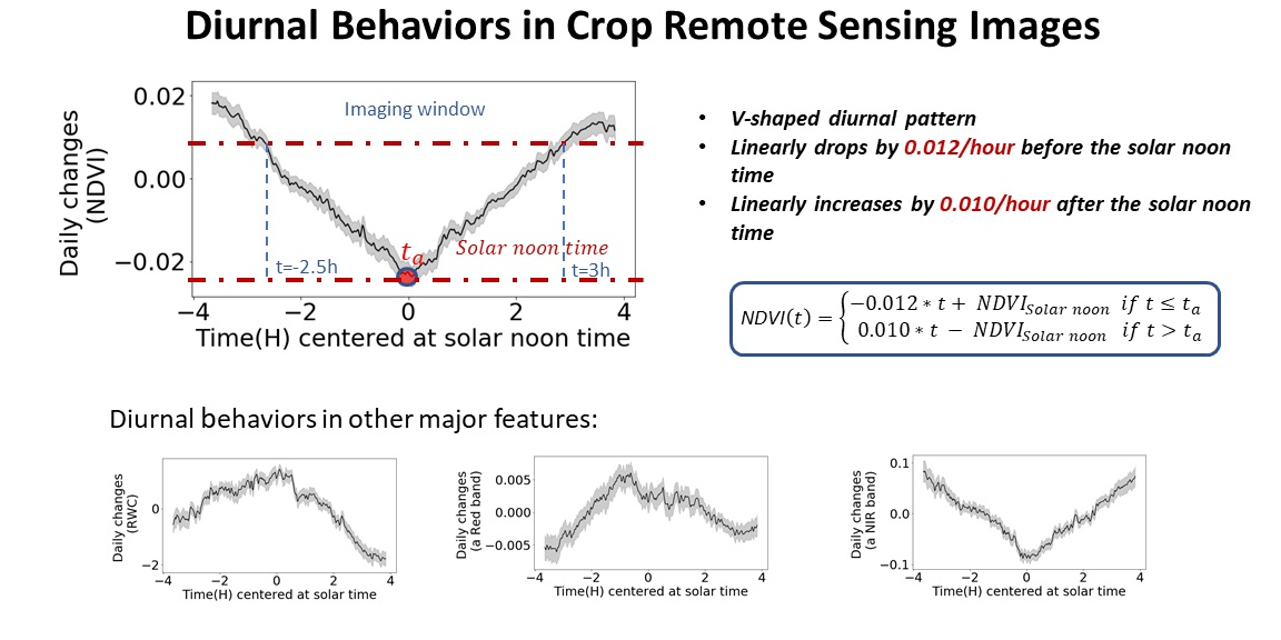
:Airborne remote sensing technologies have been widely applied in field crop phenotyping. However, the quality of current remote sensing data suffers from significant diurnal variances. The severity of the diurnal issue has been reported in various plant phenotyping studies over the last four decades, but there are limited studies on the modeling of the diurnal changing patterns that allow people to precisely predict the level of diurnal impacts. In order to comprehensively investigate the diurnal variability, it is necessary to collect time series field images with very high sampling frequencies, which has been difficult. In 2019, Purdue agricultural (Ag) engineers deployed their first field visible to near infrared (VNIR) hyperspectral gantry platform, which is capable of repetitively imaging the same field plots every 2.5 min. A total of 8631 hyperspectral images of the same field were collected for two genotypes of corn plants from the vegetative stage V4 to the reproductive stage R1 in the 2019 growing season. The analysis of these images showed that although the diurnal variability is very significant for almost all the image-derived phenotyping features, the diurnal changes follow stable patterns. This makes it possible to predict the imaging drifts by modeling the changing patterns. This paper reports detailed diurnal changing patterns for several selected plant phenotyping features such as Normalized Difference Vegetation Index (NDVI), Relative Water Content (RWC), and single spectrum bands. For example, NDVI showed a repeatable V-shaped diurnal pattern, which linearly drops by 0.012 per hour before the highest sun angle and increases thereafter by 0.010 per hour. The different diurnal changing patterns in different nitrogen stress treatments, genotypes and leaf stages were also compared and discussed. With the modeling results of this work, Ag remote sensing users will be able to more precisely estimate the deviation/change of crop feature predictions caused by the specific imaging time of the day. This will help people to more confidently decide on the acceptable imaging time window during a day. It can also be used to calibrate/compensate the remote sensing result against the time effect.
1. Introduction
Modern plant breeding efforts depend on phenotypic data to select high-yield and stress-tolerant plants quickly and efficiently [1,2]. Ag remote sensing technologies have been developing rapidly for many years. Currently, field phenotyping activities are being conducted with satellites, airborne platforms (manned and unmanned), and ground-based vehicles [3,4]. Various sensors such as RGB (Red–Green–Blue), hyperspectral and thermal cameras are carried by these platforms to take images of the crop field. These technologies have been proven effective through various Ag remote sensing projects [3,5]. However, the quality of Ag remote sensing data is still limited by various noise sources such as the changes of day light, wind speed, temperature, sun angle, etc. [6,7,8,9]. Among these noises, the diurnal variability is one of the major factors causing significant quality issues in Ag remote sensing.
The diurnal impact to plants’ reflectance characteristics is a complicated process. It introduces strong noises in plant phenotyping result [8,10,11]. For example, the reflectance characteristics of the same plants at noon can be very different from those in the afternoon. These variabilities are caused by interactions between camera’s sensitivity, camera’s view angle, canopy geometry, solar zenith angle, solar azimuth angle, and shadows [12,13]. Meanwhile, the plant itself is endogenously sensitive to the environmental conditions with the complicated interactions between the genetic backgrounds, the external environments and the treatments (G (Genotype) * E (Environment) * t (Treatment)). All these affect the final reflectance characteristics of plants throughout the day, causing the diurnal variabilities.
The diurnal variance on phenotyping data has been reported as unignorable impacts in many plant studies. Gardener [14] stated that it was a major unresolved noise issue in using reflectance measurements for estimating leaf area, plant biomass, or phenology as it was affected by diurnal changes. In the last decades, diurnal variability has been documented in various plant phenotyping studies for corn [15], soybean, wheat [11] with both passive [7,16] and active sensors [15]. These variances are retained in the captured images, weakening the signal power of the data. Sometimes, the generated variances are even larger than the plant differences caused by biotic or abiotic stresses, which severely limits the accuracy in phenotyping data [11,16]. However, for most of current remote sensing studies, people rarely consider the impacts from diurnal variabilities, which introduces severe noises into the final analysis results. For example, the NDVI values had over 10% difference at different time points on the same plant from the raw remote sensing measurements [11,16]. Similar diurnal variances are also found in many other plant features such as plant temperature, spectra features, chlorophyll content, etc. [9,17]. Therefore, it is extremely important to reduce the diurnal variabilities in the data for improved remote sensing quality.
With the development of plant phenotyping, researchers are better aware of the diurnal variabilities while there are limited studies on how to deal with diurnal variability in Ag remote sensing. To reduce impacts of diurnal variability, remote sensing technologies, such as unmanned aerial vehicles (UAV), usually have strict rules on the sampling time window and weather condition requirement [18,19,20]. According to Bellvert et al. [21], the proper time of the day to acquire thermal and multispectral images should be around noon, because there is almost complete absence of shadow effects. Meanwhile, plant physiology changes on a cyclical diurnal nature based on photosynthetic activity and processes dependent on incident solar radiation [22]. Consequently, UAV data collections are required to operate during a certain range of time for accurate monitoring crop physiology [20].
It is important to quantitatively model the diurnal variability of crop phenotyping features for improved Ag remote sensing quality. The combined PROSPECT leaf optical properties model and SAIL canopy bidirectional reflectance model (PROSAIL) has been widely used to predict the change of plant canopy spectral reflectance influenced by the changing environmental conditions such as solar angle [23,24]. However, the model does not meet the accuracy requirement in plant phenotyping remote sensing. For example, Berger et al. [25] compared PROSAIL’s simulation result with the spectra data collected from the field and found that PROSAIL’s predicted spectra showed severe drifts from the field measurements especially at the green and red edge (~700 nm) wavelengths [25]. This was also confirmed in the field remote sensing experiment in 2019 at Purdue University, in which the PROSAIL model only predicted less than 5% of the diurnal variance of the observed NDVI from a hyperspectral camera. Another potential solution arises from the use of different regression methods to predict and compensate the diurnal effects. For example, a correction model with the polynomial regression method was developed to predict the crop reflectance as a function of solar zenith angle, time of day, and ICI (instantaneous clearness index). The capability of the model in reducing the diurnal variation with Green Normalized Difference Vegetation Index (GNDVI) and some individual bands [7] was tested. However, the plant data was collected on a small portion of the leaf by a handheld radiometer with four bands, which may not properly simulate airborne remote sensing platforms carrying hyperspectral or multispectral cameras. The simple polynomial regression model could successfully describe the changes in data over three consecutive days. However, it may fail to represent the general pattern on other days when the plants are at different stages of their growth cycle. Therefore, a more accurate diurnal variability model is still urgently needed.
Modeling diurnal variability in plant phenotyping data is difficult because of the complicated interactions between plants and real-time environment conditions such as cloud coverage, wind and so on. It is necessary to collect hundreds or thousands of time series images of the same field in order to model the diurnal changes, but this had been difficult with the current airborne platforms. For instance, the UAV platforms were rarely reported to image the same field for more than one time a day due to various environmental and logistical limitations [26]. In order to solve this problem, the Ag engineers at Purdue University deployed a fixed field VNIR hyperspectral gantry platform as a “mock drone” system in Purdue’s research farm in 2019, which is similar to the phenotyping system called Terra-Ref [27]. With this field gantry imaging system, hyperspectral images of the same field can be continuously collected under various weather conditions throughout the daytime in minutely base. A local weather station and distributed soil sensors in the field provide synchronized environmental condition data with the images.
Recent advances in remote sensing technologies enable the measurement of various image-based phenotypic features such as vegetation indices (e.g., NDVI), biochemical constituents (e.g., chlorophylls), water, or raw spectral features, that dramatically boosts modern crop studies [3,28]. However, as described above, the problem of diurnal variations in these phenotypic features is still unsolved due to the limits from both hardware and software aspects. In order to close this gap, in this paper, we performed a comprehensive investigation on the diurnal variability in over 8000 repeated hyperspectral images of the same corn field taken by the field imaging gantry at Purdue University over the 2019 growing season. Images of corn plants from vegetative stage V4 to reproductive stage R1 were captured. Hyperspectral image processing algorithms were applied to calculate the reflective canopy spectra and predict plant physiological features such as NDVI, RWC, and so on. The time series decomposition method was applied to obtain diurnal curves for these plant phenotyping features. After combining the imaging results over 31 days, it clearly showed repeatable diurnal changing patterns for NDVI and other phenotyping features. Regression models were successfully developed to precisely describe these diurnal changing patterns. With the result of this work, Ag remote sensing users will be able to more precisely understand the deviation/change of crop feature predictions caused by the specific imaging time of the day. It’ll also be easier to decide on the acceptable imaging time range and calibrate the diurnal factors with the developed models.
2. Methods
2.1. High-Throughput Field Imaging Acquisition System
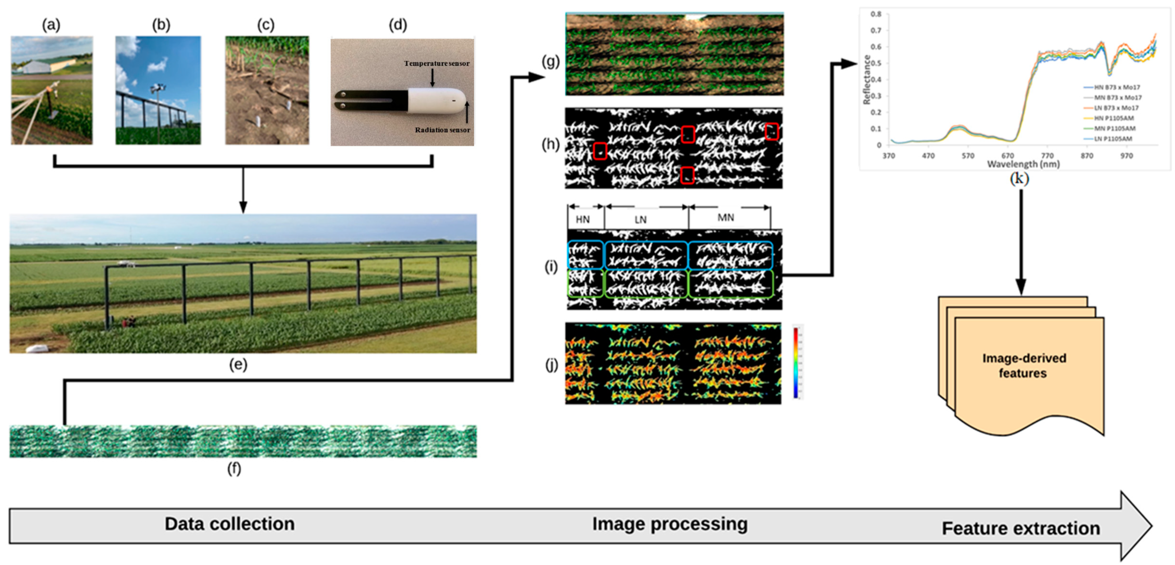
The field VNIR hyperspectral gantry platform at Purdue University’s Agronomy Center for Research and Education (ACRE) was used to collect imaging data in this study. A weatherproof VNIR push-broom hyperspectral camera (MSV-101-W, Middleton Spectral Vision, Middleton, WI, USA, Table 1) was carried by the 7 m high gantry platform to scan a 50 m by 5 m strip field under a wide range of weather conditions. The VNIR images had spectral range from 376 to 1044 nm with spectral resolution of 1.22 nm, and spatial resolution of 0.5 cm/pixel ground sample distance (GSD). The system could be configured to automatically scan the crops in the field repeatedly. It takes 6.5 min to scan the 250 square meters field, and the scanning frequency can be higher if a sub-portion of the field needed to be scanned (Figure 1).
This single sided imaging gantry stands by the north side of the field and the length of the camera structure on the top was restricted by a certain ratio of the gantry’s height. This unique design kept 100% of the shadow away from the crops. This shadow-free feature enabled the system to more realistically simulate drone remote sensing in the field. The hyperspectral camera utilizes sunlight as the lighting source, so the gantry system can function any time after sunrise until sunset on each day. A white reference panel was installed 0.5 m underneath the hyperspectral camera and moves together with it. A local mini weather station and distributed soil sensors were installed in the same field to collect real-time environmental condition data such as temperature, solar irradiation, wind speed and soil moisture when each image was taken.
2.2. Experiment Design and Data Collection
To study the diurnal variation in phenotyping data, two genotypes of corn plants, including genotype B73 × Mo17 and P1105AM, were grown in the field underneath the gantry in 2019. Each genotype was treated with three different nitrogen solutions: high nitrogen (HN) with 56 kg/ha (32 mL 28-0-0 in 1 L water), medium nitrogen (MN) with 28 kg/ha (16 mL 28-0-0 in 1 L water), and low nitrogen (LN) with 0 kg/ha (water). Each of the genotype by nitrogen treatment combination is repeated in 5 2-rows-by-3-m mini-plot replicates so there are 30 plots in total in the field (Figure 2).
In order to capture the instant impacts to the images from the changes of cloud coverage, wind speed and other environmental conditions, the team decided to have an imaging frequency of every 2.5 min. This allowed us to scan up to six different plots considering the extra time needed for data transfer, real-time image processing, and homing the gantry cart. The six plots were selected to cover all three nitrogen levels and two genotypes.
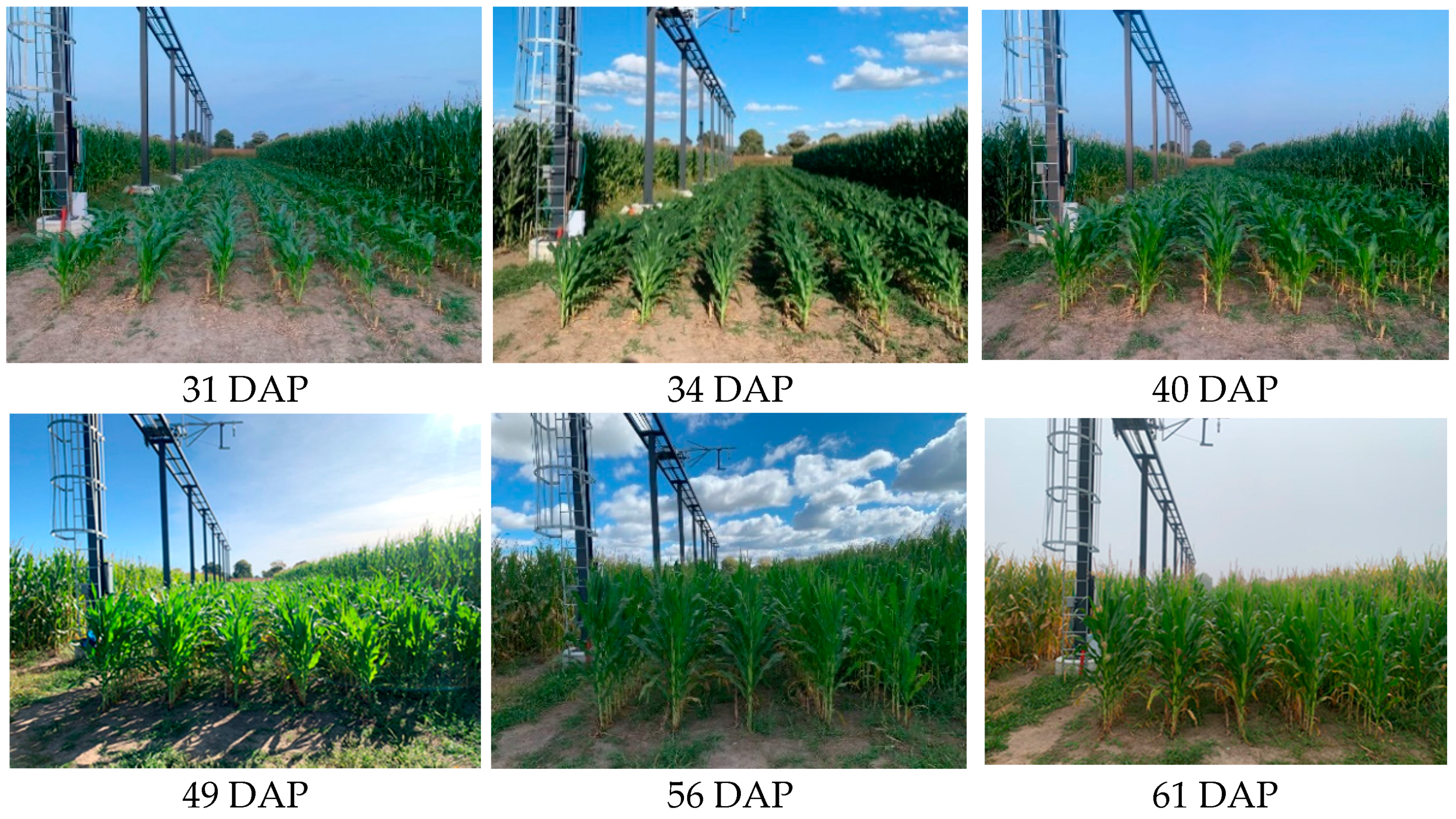
The continuous imaging started when the corn plants reached the V4 stage and lasted until 31 days later when the plants are at R1 stage on average (Figure 3). On each of the 31 days, imaging started at 8:00 a.m. and ended at 7:30 p.m. Around 280 hyperspectral images were collected with the repetitive imaging frequency of every 2.5 min. The gantry was only turned off during extreme weather conditions such as thunderstorms to protect the equipment’s safety. By the end of the 31 days, a total of 8631 hyperspectral images were collected.
In the middle of the project when the plants were at V9, we collected ground truth measurements such as nitrogen content, RWC and plant fresh weight. Two plants were randomly sampled from each plot. The plant shoot was cut to measure the fresh weight. A small section (2.5 × 5.0 cm2) of the top collared leaf was taken to measure the RWC using the Equation (1) [29,30]. The remaining part of top collared leaf was sent to the great lakes A and L laboratories (A and L Great Lakes Laboratories, Inc., Fort Wayne, IN, USA) for measuring the nitrogen percentage.
where FW is fresh weight, DW is dry weight, and TW is the turgid weight.
2.3. Image Segmentation and Feature Extraction
After data collection, standard imaging processing protocols were performed to extract the interested plant phenotyping features [5,31,32]. The raw hyperspectral images were firstly calibrated with the real-time white reference. It ensured each scanning line from this push-broom sensor was calibrated with the reference under the same lighting conditions. The image calibration was performed with the following equation:
where is the calibrated image, is the raw hyperspectral image, is dark reference image and is the hyperspectral image of the white reference. The calibrated images were then processed using a segmentation procedure with convolution methodology [33,34]. A vector of sequential integers from −20 to 20 was multiplied by the reflectance intensity vector from the red-edge region (680–720 nm). By choosing threshold 7 as the boundary, the plant tissue was successfully segmented from the background (Figure 1h). In some of images, there were some weeds which were ignorable in size compared to the corn plants (See the red boxed in Figure 1h).
The average reflectance spectrum from each plot was calculated. In total, 51,786 spectra (8631 images * 6 plots/image) were calculated for the plots with different genotypes and nitrogen treatments. These spectra were used to calculate the crop remote sensing results such as NDVI and predicted RWC. The formula below was used for calculating NDVI.
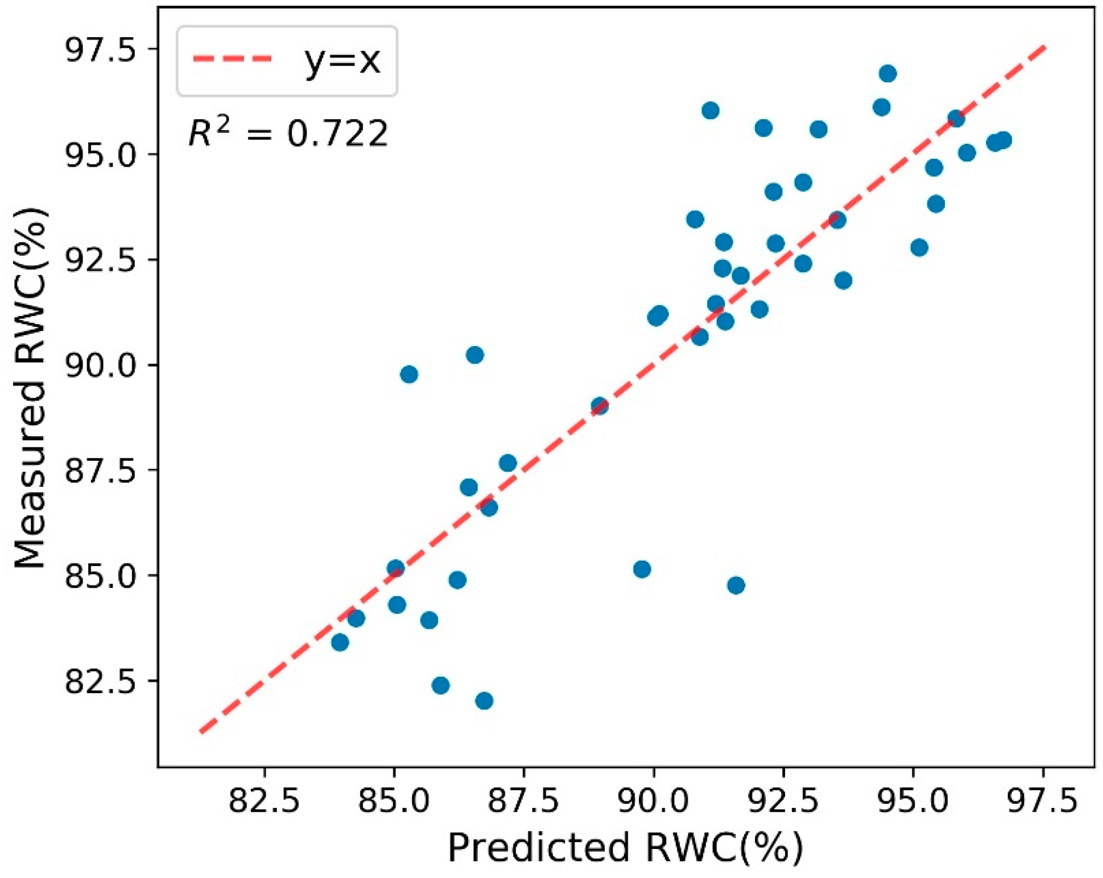
where R800nm and R650nm are the reflectance values of wavelength 800 nm and 650 nm respectively [35,36]. The partial least squares regression (PLSR) model was used to predict RWC from the spectra. In order to avoid prediction drifts between facilities [37,38,39], instead of using an existing RWC prediction model developed from the other facilities, the team decided to build a new PLSR model with the spectra and RWC ground truth data collected in the same project. The new model predicted RWC with the cross-validation coefficient of determination (R2) of 0.722 and root mean square error (RMSE) of 6.22% (Figure 4). This RWC model was then applied to all the 51,786 spectra to predict RWC in those plots over the 31 diurnal cycles.
2.4. Data Quality Check
After calculating the remote sensing result data such as spectra, NDVI and RWC, the data quality was checked, and outlier data was removed. For each feature from each day, the measurements between the upper inner fence (Q3 + 1.5IQR) and lower inner fence (Q1 − 1.5IQR) were kept [40]. IQR is the interquartile range, being equal to the difference between 75th (Q3) and 25th (Q1) percentiles. This quality filtering removed the blunders/gross errors in the image acquisition setup/process. For example, some of the removed outlier images were taken under very-high wind-speed conditions, when the plant stems were bent severely, making the images look significantly different. The data before 10:00 a.m. and after 5:30 p.m. also showed severe variances and noises. This could be caused by the dews on the surface of leaves and dim lighting conditions [41]. Only the data collected during 10 a.m.–5:30 p.m. were used in the diurnal pattern analysis as very few airborne remote sensing activities happen outside this time range. We ended up using this selected data pool (Table 2) for the diurnal pattern analysis. Please note the time was in the Eastern Time Zone Daylight Saving Time and this selected time window was actually still centered at the solar noon time in West Lafayette IN.
2.5. Evaluating the Impacts from Treatments, Stages and Genotypes to Diurnal Changing Patterns
Before modeling the diurnal changing patterns, the diurnal patterns between different nitrogen treatments, growth stages and genotypes were compared to decide if any of these factors had significant impact on the diurnal pattern. If not, the data from different treatments, stages and genotypes could be combined for the diurnal pattern modeling. Otherwise, the modeling should be done separately for each different case.
The comparison of the changing patterns was done by applying the dynamic time warping (DTW) method to calculate the similarity between the relative different ratio (RDR) curves from the different plants plots [42]. An RDR curve was calculated to describe the diurnal changing pattern on each day as the % of the change of the phenotyping feature value relative to the feature’s value at the reference time point (Equation (4)). For the reference time, we selected the solar noon time as this is the center point of the daytime, and this is when the lowest NDVI value was observed every day [11].
The DTW method was selected as it is an algorithm more commonly used to measure the similarity between two time-series data [42]. More specifically, DTW is a time series alignment algorithm developed to align two sequences of feature vectors by warping the time axis iteratively until an optimal match [43]. Thus, a distance score is generated during the process of alignment, which can be used as the difference between two curves. For example, small distance score means higher similarity between two curves. DTW also allowed non-linear mapping which was appropriate for the purpose of pattern matching. With the distance scores from DTW, the similarity of RDR curves of different plots were quantitively compared and discussed.
2.6. Diurnal Patterns Calculation by Time Series Signal Decomposition
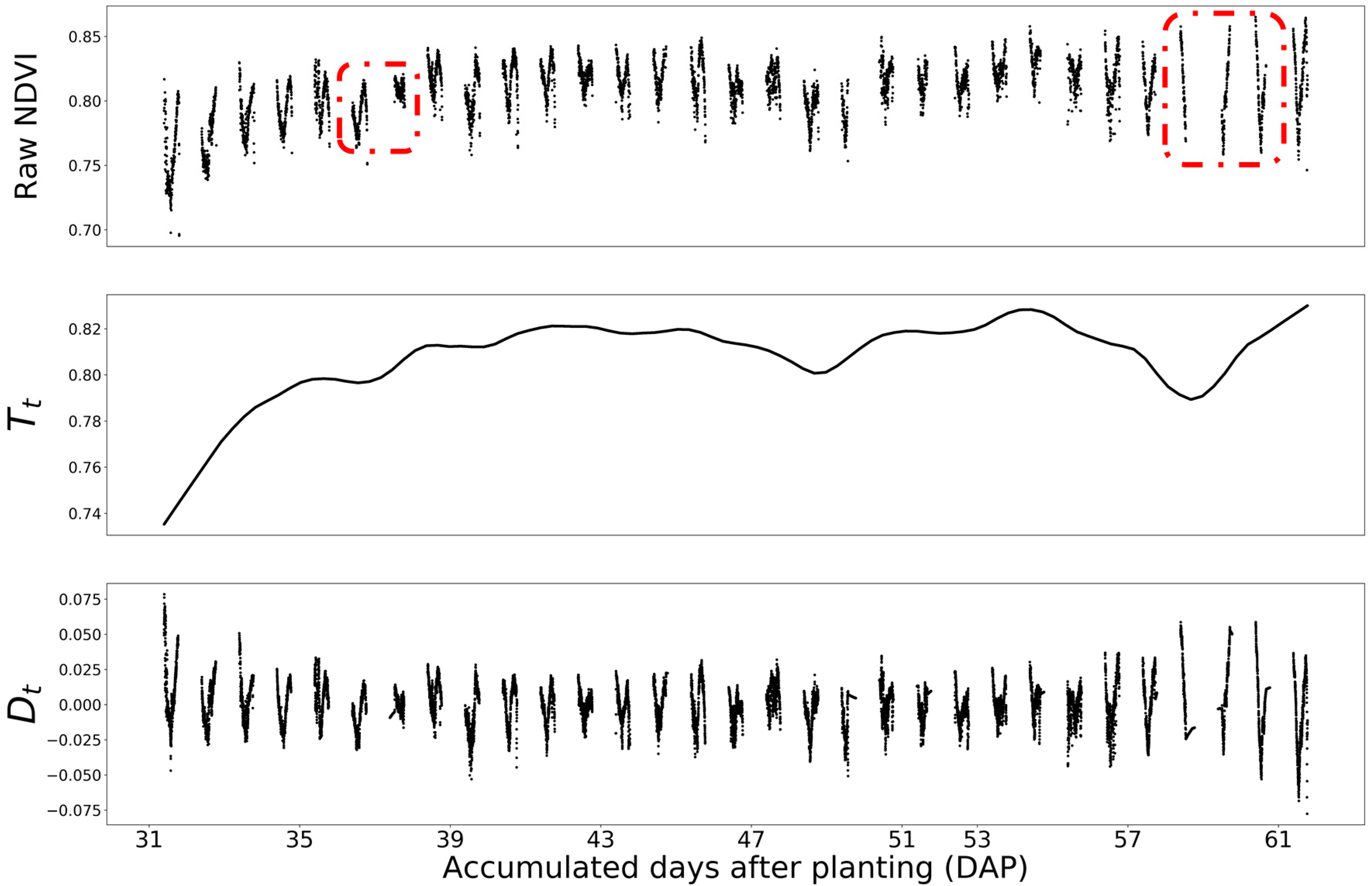
Inspired by the idea of time series decomposition method [44], we decomposed the changing signal of each feature into two major parts: day-to-day trend () and diurnal pattern (). is calculated with LOESS (locally estimated scatterplot smoothing) method [45]. By fitting a non-parametric regression curve on the scattered plot of the data, the day-to-day changing trend can be clearly extracted from the raw signal [44]. This trend is majorly reflecting the changes of plant growth stage and general weather conditions over the 31 days of imaging, which would be bothering if it is included in the diurnal pattern modeling. The diurnal component () was calculated by subtracting the day-to-day trend () from the raw signal. is also called the detrended data. contains the higher frequency variance components majorly caused by the short-term impacts such as plant’s circadian behavior, sun angle, solar irradiation and temperature changes during the day.
The mean curve of for 31 days was calculated for the diurnal pattern fitting. Meanwhile, the 95% confidence interval was also calculated to evaluate the consistency of the diurnal patterns across the days.
2.7. Diurnal Pattern Fitting
Based on the observation for the diurnal changing pattern of NDVI, a piecewise linear regression function was selected to fit the pattern. By calculating the 1st order derivative of the mean curve, the critical lowest point (which perfectly matched the time with the highest sun angle) was derived.
where t is the time offset (in hours) from solar noon. (i.e., t at 12:15 pm is -1.5, on a day and at a location where solar noon is 13:45.).
Non-linear diurnal changing patterns were observed for the other features such as RWC prediction and a few single spectral bands. We selected the 2nd order regression model (Equation (7)) for fitting the pattern of those features.
2.8. Model Performance Evaluation
The performance of the developed diurnal model was evaluated and compared with the R2 and RMSE between the prediction results and the desired diurnal changes. Moreover, to further assess the impacts from nitrogen treatments and genotypes, the general diurnal model was tested on each of the six plant plots, and the R2 and RMSE were obtained for each plot, respectively.
2.9. Diurnal Models’ Applications
These regression models quantitively summaries the diurnal impacts. For one example, the models can be used to calculate the exact imaging window based on any specific diurnal variance requirement. Besides, the models can also be used to remove the diurnal impact. For example, the NDVI measured at any other time point of the day can be converted to the NDVI at the highest sun angle time with the fitted model.
3. Results
In this study, the diurnal changing patterns models were built for various plant phenotyping features (including NDVI, RWC, Band670 (Red) and Band760 (NIR)). The detailed procedures and corresponding results for modeling NDVI’s diurnal changing pattern was demonstrated and discussed first, as NDVI is one of the most common plant features in remote sensing [46]. The summarized modeling results are reported for the other plant phenotyping features including RWC, Red and NIR, respectively.
3.1. The NDVI Diurnal Fluctuations
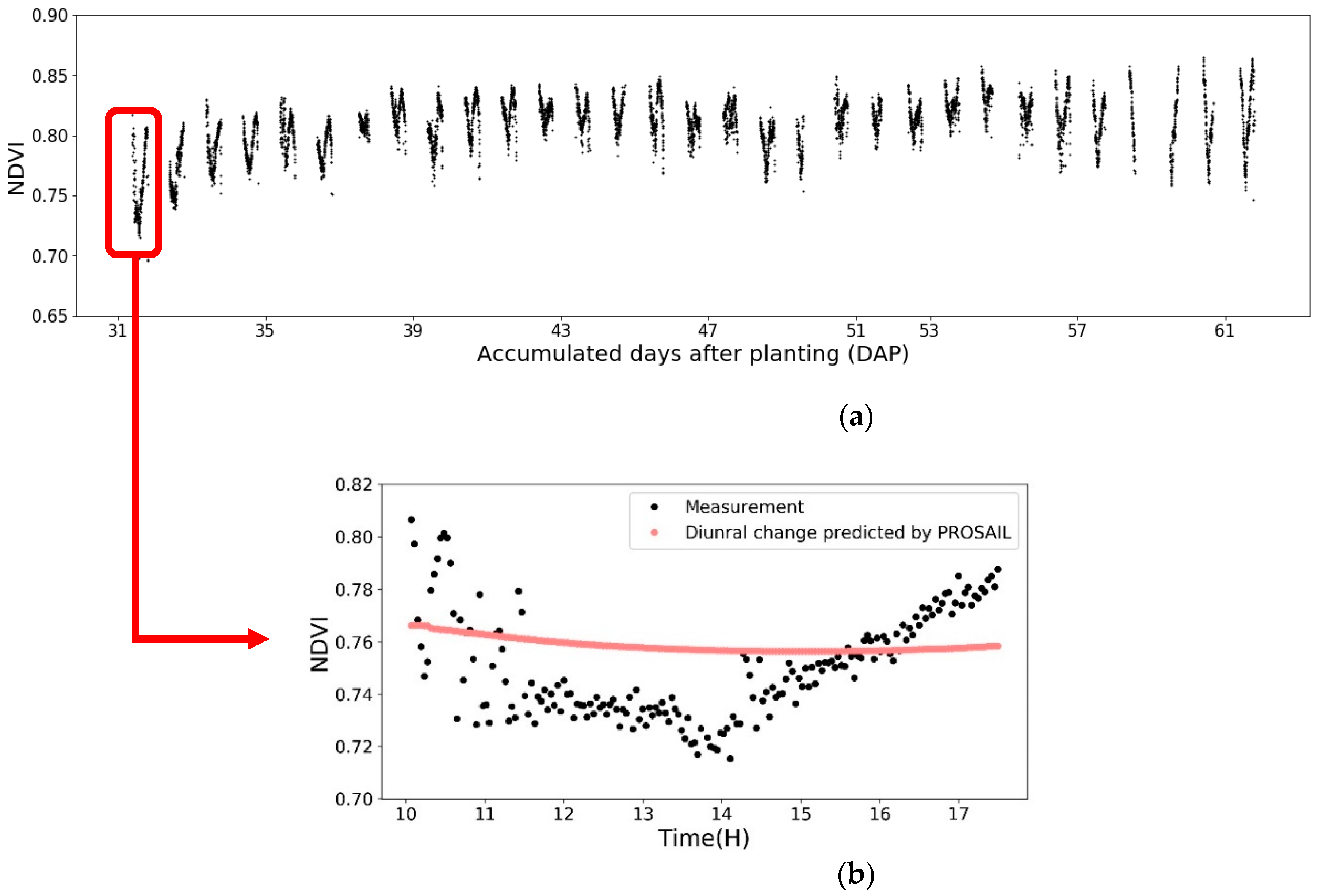
The change of NDVI values was plotted to show the diurnal fluctuations from the raw imaging data (Figure 5). Figure 5a is the result for all 31 days. Each gathering group represents one day, and the gaps between groups are from 17:30 until 10:00 next day without imaging data. In this figure, NDVI shows obvious diurnal variabilities with repeatable V-shaped patterns. Figure 5b is the zoomed in diurnal fluctuation in Day 1. It shows that NDVI keeps decreasing until the solar noon time at 1:39 p.m. on that day. This confirmed the similar findings were reported in previous research papers that the NDVI of wheat and soybean were higher at the beginning and end of the day [16,47]. This diurnal change could be due to the combination of the imaging lighting condition change and the plant’s physiology changes on a cyclical diurnal nature, which is a central behavior to regulate the susceptibility and responses to biotic or abiotic stresses [48,49,50].
The significance of diurnal variance was assessed by calculating the difference ratio between highest and lowest NDVI during the same day (Table 3). NDVI had the highest diurnal variance of 15.71% for the HN and B73 × Mo17 genotype plot. This high diurnal variance is too severe to be accepted in most plant phenotyping studies [51,52]. This justifies the needs to model the diurnal pattern and calibrate the diurnal impacts.
3.2. The Impacts of Nutrient Treatments, Genotypes and Leaf Stages on Diurnal Variation
The relative difference ratio (RDR) curves were compared to study the impacts from treatments, genotypes and growth stages on diurnal variation patterns. For each plant plot, the mean RDR curve was computed from all the 31 RDR curves (one RDR curve per day). In Figure 6, the mean RDR curves from different treatments and genotype plots showed very similar changing patterns.
For a more quantitative comparison, the DTW distance scores were calculated to measures the similarity between RDR curves (Table 4). Small distance score means higher similarity between two curves. The distance scores between plots with the same genotype but different nitrogen treatments are between 1.37~3.75. Meanwhile, the distance scores between different genotype plots are 0.33, 0.20 and 0.30 for HN, MN and LN, respectively. Table 5 recorded the DTW distance scores between different leaf stages. Most of these distance scores are below 1. As a summary, comparatively, the nitrogen treatment had higher impact on the diurnal variation than genotype and plant stage. This confirmed the observation in previous study [53]. However, all these factors had minor impacts on the diurnal changing pattern. This allowed to combine the data for building one general diurnal changing model.
3.3. Diurnal Changing Pattern
Based on the result in Section 3.2, the data of all six plant plots were combined for modeling the diurnal changing pattern because the nitrogen treatments, genotypes and leaf stages only had minor impacts on the diurnal variation and a general diurnal pattern model is preferred for ease of use.
3.3.1. Decomposition
The changing signal of phenotyping features were decomposed into two major parts: day-to-day trend () and diurnal pattern (). Figure 7 shows the decomposition result for NDVI. From the trend chart, the overall NDVI values increased from the early leaf stage to the late stage. This confirmed with the expectation that as plants grew up, NDVI increases until the reproductive stage [54]. Meanwhile, there were two big dips along the timeline, which matched well with two severe temperature drops in the West Lafayette area. Therefore, the day-to-day trend well described the changes of plant stage and plant health conditions.
On the other hand, the diurnal pattern chart in Figure 7 showed clear periodical oscillation with repeated V-shapes. For most days, the diurnal patterns were substantially consistent that the value decreased until reaching the solar noon time. We were not able to collect the complete data for the whole day on 36, 37, 58, 59 and 60 DAP due to the extreme weather conditions. It is interesting to investigate how the real-time weather conditions affect phenotyping results at different leaf stages. In this paper, we only focus on modeling the diurnal changing patterns under “normal” weather conditions. The modeling of the weather condition impacts will be reported in another paper.
To model the general diurnal pattern, the patterns through the 31 days were combined for the mean curve and 95% confidence interval (Figure 8). The narrow 95% confidence interval also provided strong evidence that the diurnal pattern is consistent through the days. As discussed in the methods, because the confidence interval is much lower compared with the mean curve’s change over the diurnal cycle, the mean curve (black line) is used for modeling the diurnal pattern. This also helps to “average out” the impacts from abnormal weather conditions in a few certain days.
3.3.2. Pattern Fitting
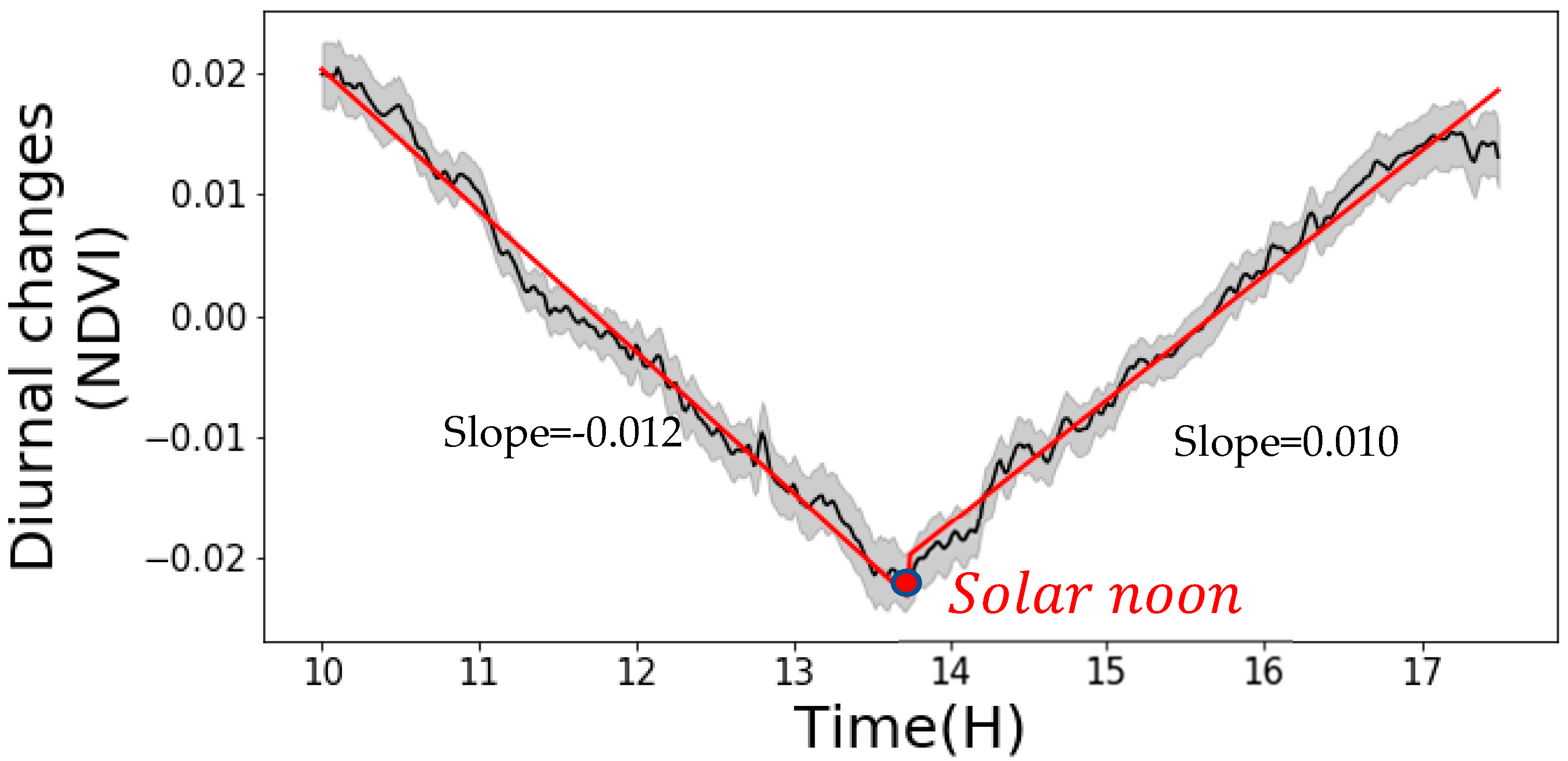
Both 1st order and 2nd order piecewise models were tested to fit the diurnal pattern of NDVI. Both had excellent regression performances and there was no significant difference between the two models. Therefore, we adopted the simpler 1st order model, and we concluded that the NDVI diurnal changing pattern can be described by a linear model. The fitting equations in Equation (8) accurately predicted the observed diurnal pattern. The predicted NDVI values and the measured values had R2 of 0.99 and RMSE of 0.0012. Figure 8 illustrates the detailed fitted result. To test the validation of the model for different genotypes and nitrogen treatments, the fitted equation was applied on each different field plot, respectively. The model maintained accurate performance in all cases (Table 6). It proves this general diurnal pattern model is valid for plants from different nutrient treatments and genotypes.
It can be noted that the critical time in Equation (8) is 13:42, which is within the actual solar noon time ranging from 13:35 to 13:45. Therefore, we conclude that the solar angel is one of the major impacts to the diurnal variance, so Equation (8) should be shifted based on the actual solar noon time on each day (replacing “13:42” in Equation (8) with the actual solar noon time on the imaging day).
where t is the time offset (in hours) from solar noon. (i.e., t at 12:15 pm is -1.5, on a day and at a location where solar noon is 13:45.) is the NDVI measured at solar noon.
3.3.3. Applications of the Model
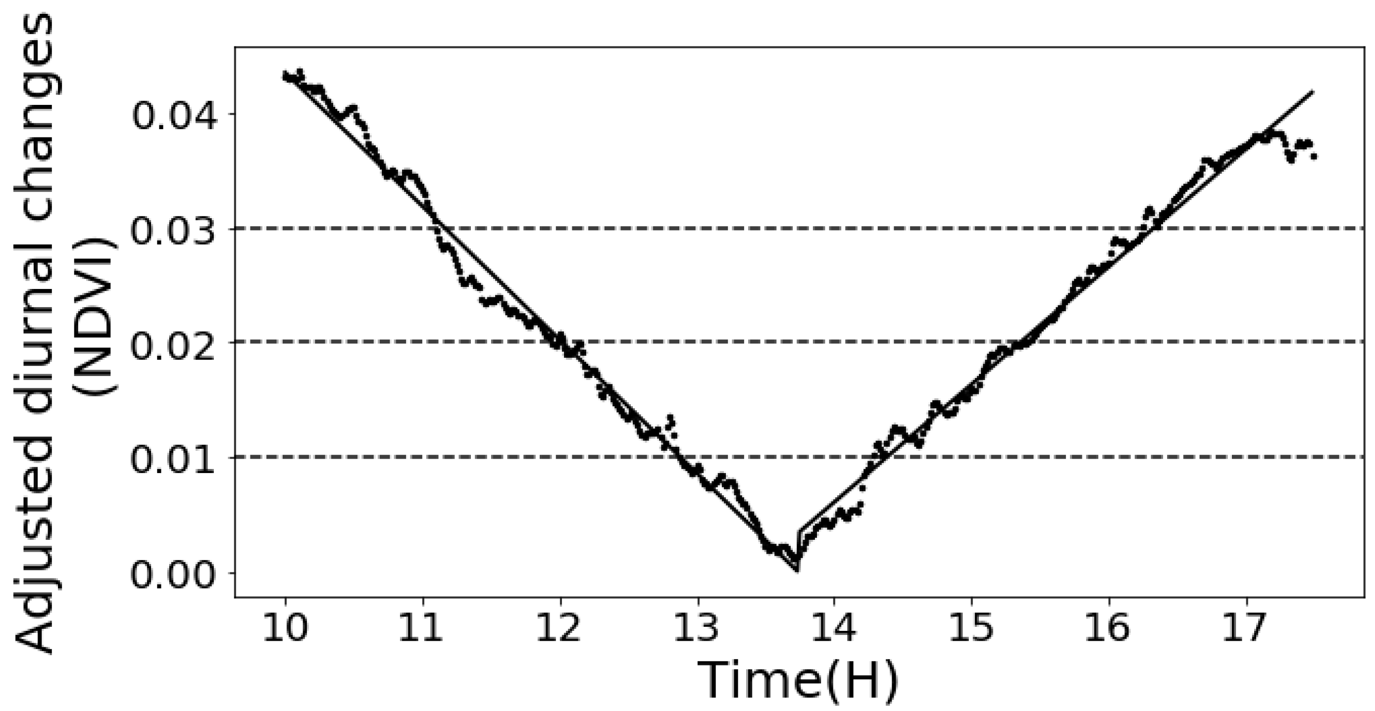
The diurnal changing pattern model can be utilized to determine the proper imaging window based on any specific quality requirement. In Figure 9 and Table 7, the proper imaging windows were calculated based on the different thresholds tolerated diurnal variance. For example, in order to control the NDVI’s diurnal error within ±0.03, the imaging needs to happen between 10:55 and 16:30.
Besides the imaging time window, the diurnal changing model can also be used to easily calibrate the diurnal variances. For example, the NDVI measured 2 h before the solar noon time should be decreased by 0.024 (0.012 * 2), so the calibrated NDVI is as if it is taken exactly at the solar noon time. It’ll be important to run this calibration process, which will help to remove the significant diurnal variance and enable phenotyping researchers to do “apple-to-apple” comparison between the NDVIs of the different plots.
3.4. Other Image-Derived Phenotyping Features
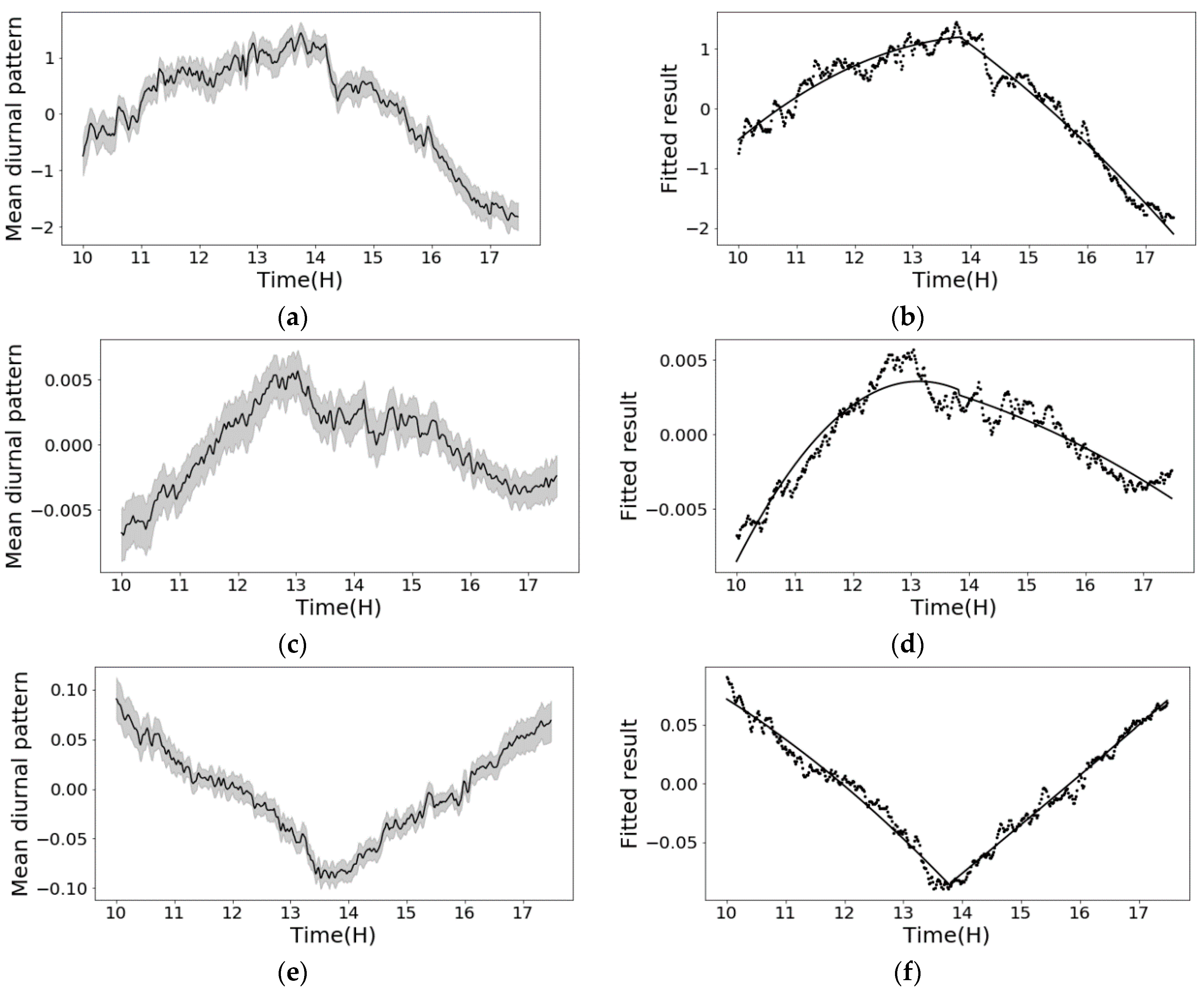
Besides NDVI, the diurnal changing patterns of other plant phenotyping features, including RWC prediction, Red and NIR in the spectra, were modeled. From Figure 10a,c,e, the result showed consistent diurnal patterns of these features with clear mean curve and narrow 95% CI.
Second order models were selected, because these other features showed non-linear diurnal changing patterns. The diurnal patterns were fitted and plotted in Figure 10b,d,f. Equations (9)–(11) are the fitted equations. All the models showed excellent description of the observed diurnal patterns. The R2 and RMSE between the models’ prediction and the measured features are summarized in Table 8. Similarly, these models have the potential to help improving the efficiency and data quality in phenotyping practices. Moreover, successful application of the same proposed diurnal pattern modelling method on the RWC, Red and NIR indicated that this method has potential to be generalized well on other phenotypic features which can be further explored.
4. Discussions
4.1. Strengths
Benefited from the unprecedented high imaging frequency of the new field hyperspectral imaging gantry at Purdue, with over eight thousand repeated images over one growing season, the detailed diurnal patterns of plant phenotyping features, including NDVI, RWC, and two individual spectral bands (Red and NIR), were quantitatively described and modeled for the first time. Moreover, most of previous studies reported the diurnal changes directly from the raw phenotyping features (e.g., NDVI, chlorophyll content) [11,16,23]. However, these results are inconsistent due to the changes of plant growth stage and weather condition. To address this issue, our proposed approach incorporates a modified time series decomposition method to filter out the signal variance caused by the changing plant stage and weather conditions, so the later modeling process can exclusively focus on the higher-frequency diurnal changes.
4.2. Limitations and Future Work
In this experiment, all the imaging data was collected from the same field imaging gantry facility. Extra validation is needed for the other remote sensing platforms such as UAV. In addition, the diurnal patterns are reported based on corn plants, which may limit the scope of application. It is necessary to conduct more tests including more diverse plant species (e.g., soybean, wheat, and rice).
In the 2020 season, the developed diurnal models will be externally validated with the field gantry’s images. The model will also be validated on a UAV hyperspectral imaging platform in the same field. Finally, the diurnal changing patterns on other plant species, such as soybean wheat, and rice will be also explored and compared.
Besides the diurnal effect, the changing environmental conditions in the field such as cloud coverage, temperature, wind speed and so on all showed strong impacts on the phenotyping results. The data has shown that these effects could be precisely modeled as well. The environmental calibration models for plant remote sensing will be reported in future papers.
5. Conclusions
In this study, diurnal changing patterns in crop remote sensing images were quantitatively investigated with the proposed novel modeling approach. The diurnal patterns for four selected plant phenotyping features, including NDVI, RWC, two individual spectral bands (Red and NIR), were successfully modeled. The results showed that the NDVI presents a repeatable V-shaped diurnal changing pattern: it linearly decreases by 0.012/h before the solar noon time and increases by 0.010/h thereafter. On the other hand, the RWC, and the two individual spectral bands shows non-linear diurnal changing patterns, where RWC and Red change in inversed V-shaped patterns, and NIR changes in a normal V-shaped pattern. The diurnal patterns lightly vary between the nitrogen treatments, genotypes, and plant stages, but the difference is minor and ignorable in the modeling. With the result of this work, Ag remote sensing users will be able to more precisely understand the deviation/change of crop feature predictions caused by the specific imaging time of the day. The reported diurnal models can also be used to calibrate the remote sensing result so to remove the diurnal impacts.
Author Contributions
D.M. carried out the data collection, data analysis, and drafted the manuscript; J.J. contributed the research idea, led the designing, fund-raising and construction of the field imaging facility, designed the experiments and revised the manuscript; H.M. and M.R.T. guided the experimental design; T.U.R. and L.Z. made substantial contributions to system construction and data collection. All authors have read and agreed to the published version of the manuscript.
Funding
This research was funded by Sumitomo Chemical, grant number 16121941 and The APC was funded by Purdue University.
Data Availability Statement
The data presented in this study are available on request from the corresponding author. The data are not publicly available due to confidentiality.
Acknowledgments
The project was sponsored and supported by Sumitomo Chemical and Department of Agricultural and Biological Engineering, Purdue University. The authors would like to thank Meng-Yang Lin (Student, Department of Agronomy, Purdue University) for his assistance in ground truth data collection.
Conflicts of Interest
The authors declare no conflict of interest.
References
- Houle, D.; Govindaraju, D.R.; Omholt, S. Phenomics: The next challenge. Nat. Rev. Genet. 2010, 11, 855–866. [Google Scholar] [CrossRef]
- Fiorani, F.; Schurr, U. Future Scenarios for Plant Phenotyping. Annu. Rev. Plant. Biol. 2013, 64, 267–291. [Google Scholar] [CrossRef] [PubMed] [Green Version]
- Li, L.; Zhang, Q.; Huang, D. A Review of Imaging Techniques for Plant Phenotyping. Sensors 2014, 20078–20111. [Google Scholar] [CrossRef] [PubMed]
- Rehman, T.U.; Mahmud, M.S.; Chang, Y.K.; Jin, J.; Shin, J. Current and future applications of statistical machine learning algorithms for agricultural machine vision systems. Comput. Electron. Agric. 2019, 156, 585–605. [Google Scholar] [CrossRef]
- Wang, L.; Jin, J.; Song, Z.; Wang, J.; Zhang, L.; Rehman, T.U.; Ma, D.; Carpenter, N.R.; Tuinstra, M.R. LeafSpec: An accurate and portable hyperspectral corn leaf imager. Comput. Electron. Agric. 2020, 169, 105209. [Google Scholar] [CrossRef]
- Fiorani, F.; Rascher, U.; Jahnke, S.; Schurr, U. Imaging plants dynamics in heterogenic environments. Curr. Opin. Biotechnol. 2012, 23, 227–235. [Google Scholar] [CrossRef]
- de Souza, E.G.; Scharf, P.C.; Sudduth, K.A. Sun position and cloud effects on reflectance and vegetation indices of corn. Agron. J. 2010, 102, 734–744. [Google Scholar] [CrossRef] [Green Version]
- Maji, S.; Chandra, B.; Viswavidyalaya, K. Diurnal Variation in Spectral Properties of Potato under Different Dates of Planting and N-Doses. Environ. Ecol. 2015, 33, 478–483. [Google Scholar]
- Gamon, J.A.; Kovalchuck, O.; Wong, C.Y.S.; Harris, A.; Garrity, S.R. Monitoring seasonal and diurnal changes in photosynthetic pigments with automated PRI and NDVI sensors. Biogeosciences 2015, 12, 4149–4159. [Google Scholar] [CrossRef] [Green Version]
- Padilla, F.M.; de Souza, R.; Peña-Fleitas, M.T.; Grasso, R.; Gallardo, M.; Thompson, R.B. Influence of time of day on measurement with chlorophyll meters and canopy reflectance sensors of different crop N status. Precis. Agric. 2019, 20, 1087–1106. [Google Scholar] [CrossRef] [Green Version]
- Beneduzzi, H.M.; Souza, E.G.; Bazzi, C.L.; Schenatto, K. Temporal variability in active reflectance sensor-measured NDVI in soybean and wheat crops. Eng. Agric. 2017, 37, 771–781. [Google Scholar] [CrossRef]
- Ranson, K.J.; Daughtry, C.S.T.; Biehl, L.L.; Bauer, M.E. Sun-view angle effects on reflectance factors of corn canopies. Remote Sens. Environ. 1985. [Google Scholar] [CrossRef]
- Jackson, R.D.; Pinter, P.J., Jr.; Idso, S.B.; Reginato, R.J. Wheat spectral reflectance: Interactions between crop configuration, sun elevation, and azimuth angle. Appl. Opt. 1979, 18, 3730–3732. [Google Scholar] [CrossRef] [PubMed]
- Gardner, B.R. Techniques for Remotely Monitoring Canopy Development and Estimating Grain Yield of Moisture Stressed Corn (Landsat, Sensed). Ph.D. Thesis, University of Nebraska-Lincoln, Lincoln, NE, USA, 1983. Available online: https://digitalcommons.unl.edu/dissertations/AAI8412302 (accessed on 26 April 2021).
- Oliveira, L.F.; Scharf, P.C. Diurnal variability in reflectance measurements from cotton. Crop. Sci. 2014, 54, 1769–1781. [Google Scholar] [CrossRef]
- Sticksel, E.; Schächtl, J.; Huber, G.; Liebler, J.; Maidl, F.X. Diurnal variation in hyperspectral vegetation indices related to winter wheat biomass formation. Precis. Agric. 2004, 5, 509–520. [Google Scholar] [CrossRef]
- Zhao, L.; Liu, Z.; Xu, S.; He, X.; Ni, Z.; Zhao, H.; Ren, S. Retrieving the diurnal FPAR of a maize canopy from the jointing stage to the tasseling stage with vegetation indices under different water stresses and light conditions. Sensors 2018, 18, 3965. [Google Scholar] [CrossRef] [Green Version]
- Di Gennaro, S.F.; Rizza, F.; Badeck, F.W.; Berton, A.; Delbono, S.; Gioli, B.; Toscano, P.; Zaldei, A.; Matese, A. UAV-based high-throughput phenotyping to discriminate barley vigour with visible and near-infrared vegetation indices. Int. J. Remote Sens. 2018, 39, 5330–5344. [Google Scholar] [CrossRef]
- Gracia-Romero, A.; Kefauver, S.C.; Fernandez-Gallego, J.A.; Vergara-Díaz, O.; Nieto-Taladriz, M.T.; Araus, J.L. UAV and ground image-based phenotyping: A proof of concept with durum wheat. Remote Sens. 2019, 11, 1244. [Google Scholar] [CrossRef] [Green Version]
- Barbedo, J.G.A. A Review on the Use of Unmanned Aerial Vehicles and Imaging Sensors for Monitoring and Assessing Plant Stresses. Drones 2019, 3, 40. [Google Scholar] [CrossRef] [Green Version]
- Bellvert, J.; Girona, J. The use of multispectral and thermal images as a tool for irrigation scheduling in vineyards. Use Remote. Sens. Geogr. Inf. Syst. Irrig. Manag. Southwest Eur. 2012, 137, 131–137. [Google Scholar]
- Campbell, P.K.E.; Huemmrich, K.F.; Middleton, E.M.; Ward, L.A.; Julitta, T.; Daughtry, C.S.T.; Burkart, A.; Russ, A.L.; Kustas, W.P. Diurnal and seasonal variations in chlorophyll fluorescence associated with photosynthesis at leaf and canopy scales. Remote Sens. 2019, 11, 488. [Google Scholar] [CrossRef] [Green Version]
- Ishihara, M.; Inoue, Y.; Ono, K.; Shimizu, M.; Matsuura, S. The impact of sunlight conditions on the consistency of vegetation indices in croplands-Effective usage of vegetation indices from continuous ground-based spectral measurements. Remote Sens. 2015, 7, 14079–14098. [Google Scholar] [CrossRef] [Green Version]
- Jacquemoud, S.; Baret, F. PROSPECT: A model of leaf optical properties spectra. Remote Sens. Environ. 1990, 34, 75–91. [Google Scholar] [CrossRef]
- Berger, K.; Atzberger, C.; Danner, M.; Wocher, M.; Mauser, W.; Hank, T. Model-based optimization of spectral sampling for the retrieval of crop variables with the PROSAIL model. Remote Sens. 2018, 10, 2063. [Google Scholar] [CrossRef] [Green Version]
- Krishna, K.R. Agricultural Drones: A Peaceful Pursuit; CRC Press: Boca Raton, FL, USA, 2018. [Google Scholar]
- Burnette, M.; Kooper, R.; Maloney, J.D.; Rohde, G.S.; Terstriep, J.A.; Willis, C.; Fahlgren, N.; Mockler, T.; Newcomb, M.; Sagan, V.; et al. TERRA-REF data processing infrastructure. In Proceedings of the Practice and Experience on Advanced Research Computing, Pittsburgh, PA, USA, 22–26 July 2017; pp. 1–7. Available online: https://dl.acm.org/doi/abs/10.1145/3219104.3219152 (accessed on 26 April 2021).
- Pandey, P.; Ge, Y.; Stoerger, V.; Schnable, J.C. High throughput in vivo analysis of plant leaf chemical properties using hyperspectral imaging. Front. Plant. Sci. 2017, 8, 1–12. [Google Scholar] [CrossRef] [PubMed] [Green Version]
- Turner, N.C. Techniques and experimental approaches for the measurement of plant water status. Plant Soil 1981, 58, 339–366. [Google Scholar] [CrossRef]
- Ma, D.; Carpenter, N.; Maki, H.; Rehman, T.U.; Tuinstra, M.R.; Jin, J. Greenhouse environment modeling and simulation for microclimate control. Comput. Electron. Agric. 2019, 162, 134–142. [Google Scholar] [CrossRef]
- Ma, D.; Maki, H.; Neeno, S.; Zhang, L.; Wang, L.; Jin, J. Application of non-linear partial least squares analysis on prediction of biomass of maize plants using hyperspectral images. Biosyst. Eng. 2020, 200, 40–54. [Google Scholar] [CrossRef]
- Ma, D.; Wang, L.; Zhang, L.; Song, Z.; Rehman, T.U.; Jin, J. Stress distribution analysis on hyperspectral corn leaf images for improved phenotyping quality. Sensors 2020, 20, 3659. [Google Scholar] [CrossRef]
- Zhang, L.; Maki, H.; Ma, D.; Sánchez-Gallego, J.A.; Mickelbart, M.V.; Wang, L.; Rehman, T.U.; Jin, J. Optimized angles of the swing hyperspectral imaging system for single corn plant. Comput. Electron. Agric. 2019, 156, 349–359. [Google Scholar] [CrossRef]
- Ma, D.; Carpenter, N.; Amatya, S.; Maki, H.; Wang, L.; Zhang, L.; Neeno, S.; Tuinstra, M.R.; Jin, J. Removal of greenhouse microclimate heterogeneity with conveyor system for indoor phenotyping. Comput. Electron. Agric. 2019, 166, 104979. [Google Scholar] [CrossRef]
- Schafleitner, R.; Gutierrez, R.; Espino, R.; Gaudin, A.; Pérez, J.; Martínez, M.; Domínguez, A.; Tincopa, L.; Alvarado, C.; Numberto, G.; et al. Field screening for variation of drought tolerance in Solanum tuberosum L. by agronomical, physiological and genetic analysis. Potato Res. 2007, 50, 71–85. [Google Scholar] [CrossRef]
- Daughtry, C.S.T.; Walthall, C.L.; Kim, M.S.; De Colstoun, E.B.; McMurtrey Iii, J.E. Estimating corn leaf chlorophyll concentration from leaf and canopy reflectance. Remote Sens. Environ. 2000, 74, 229–239. [Google Scholar] [CrossRef]
- Alamar, M.C.; Bobelyn, E.; Lammertyn, J.; Nicolaï, B.M.; Moltó, E. Calibration transfer between NIR diode array and FT-NIR spectrophotometers for measuring the soluble solids contents of apple. Postharvest Biol. Technol. 2007, 45, 38–45. [Google Scholar] [CrossRef]
- Ji, W.; Viscarra Rossel, R.A.; Shi, Z. Improved estimates of organic carbon using proximally sensed vis-NIR spectra corrected by piecewise direct standardization. Eur. J. Soil Sci. 2015, 66, 670–678. [Google Scholar] [CrossRef]
- Li, X.; Cai, W.; Shao, X. Correcting multivariate calibration model for near infrared spectral analysis without using standard samples. J. Near Infrared Spectrosc. 2015, 23, 285–291. [Google Scholar] [CrossRef]
- Schwertman, N.C.; de Silva, R. Identifying outliers with sequential fences. Comput. Stat. Data Anal. 2007. [Google Scholar] [CrossRef]
- Manea, D.; Calin, M.A. Hyperspectral imaging in different light conditions. Imaging Sci. J. 2015, 63, 214–219. [Google Scholar] [CrossRef]
- Berndt, D.; Clifford, J. Using dynamic time warping to find patterns in time series. Work. Knowl. Knowl. Discov. Databases 1994, 398, 359–370. [Google Scholar]
- Kate, R.J. Using dynamic time warping distances as features for improved time series classification. Data Min. Knowl. Discov. 2016, 30, 283–312. [Google Scholar] [CrossRef]
- Cleveland, R.B.; Cleveland, W.S.; McRae, J.E.; Terpenning, I. STL: A seasonal-trend decomposition. J. Off. Stat. 1990, 6, 3–73. [Google Scholar]
- Rojo, J.; Rivero, R.; Romero-Morte, J.; Fernández-González, F.; Pérez-Badia, R. Modeling pollen time series using seasonal-trend decomposition procedure based on LOESS smoothing. Int. J. Biometeorol. 2017, 61, 335–348. [Google Scholar] [CrossRef] [PubMed]
- Cabrera-Bosquet, L.; Molero, G.; Stellacci, A.; Bort, J.; Nogués, S.; Araus, J. NDVI as a potential tool for predicting biomass, plant nitrogen content and growth in wheat genotypes subjected to different water and nitrogen conditions. Cereal Res. Commun. 2011, 39, 147–159. [Google Scholar] [CrossRef]
- Sagan, V.; Maimaitijiang, M.; Sidike, P.; Maimaitiyiming, M.; Erkbol, H.; Hartling, S.; Peterson, K.T.; Peterson, J.; Burken, J.; Fritschi, F. Uav/satellite multiscale data fusion for crop monitoring and early stress detection. Int. Arch. Photogramm. Remote Sens. Spat. Inf. Sci. 2019, 42, 715–722. [Google Scholar] [CrossRef] [Green Version]
- Dunford, R.P.; Yano, M.; Kurata, N.; Sasaki, T.; Huestis, G.; Rocheford, T.; Laurie, D.A. Comparative mapping of the barley Ppd-H1 photoperiod response gene region, which lies close to a junction between two rice linkage segments. Genetics 2002, 161, 825–834. [Google Scholar] [CrossRef] [PubMed]
- Kloosterman, B.; Abelenda, J.A.; Gomez, M.D.M.C.; Oortwijn, M.; De Boer, J.M.; Kowitwanich, K.; Horvath, B.M.; Van Eck, H.J.; Smaczniak, C.; Prat, S.; et al. Naturally occurring allele diversity allows potato cultivation in northern latitudes. Nature 2013, 495, 246–250. [Google Scholar] [CrossRef] [PubMed]
- Turner, A. The Pseudo-Response Regulator Ppd-H1 Provides The Pseudo-Response Regulator Ppd-H1 Provides Adaptation to Photoperiod in Barley. Science 2007, 1031, 1031–1035. [Google Scholar] [CrossRef]
- Ni, Z.; Liu, Z.; Huo, H.; Li, Z.L.; Nerry, F.; Wang, Q.; Li, X. Early water stress detection using leaf-level measurements of chlorophyll fluorescence and temperature data. Remote Sens. 2015, 7, 3232–3249. [Google Scholar] [CrossRef] [Green Version]
- Rahman, M.M.; Lamb, D.W.; Stanley, J.N. The impact of solar illumination angle when using active optical sensing of NDVI to infer fAPAR in a pasture canopy. Agric. Meteorol. 2015, 202, 39–43. [Google Scholar] [CrossRef]
- Atkin, O.K.; Holly, C.; Ball, M.C. Acclimation of snow gum (Eucalyptus pauciflora) leaf respiration to seasonal and diurnal variations in temperature: The importance of changes in the capacity and temperature sensitivity of respiration. Plant Cell Environ. 2000, 23, 15–26. [Google Scholar] [CrossRef]
- Wang, R.; Cherkauer, K.; Bowling, L. Corn Response to Climate Stress Detected with Satellite-Based NDVI Time Series. Remote. Sens. 2016, 8, 269. [Google Scholar] [CrossRef] [Green Version]
Figure 1.
Field VNIR hyperspectral platform at Purdue University. (a) VNIR hyperspectral imaging sensor; (b) Local weather station (Ambient Weather, Chandler, AZ, USA); (c,d) Xiaomi flower care sensor (Xiaomi Inc., Beijing, China); (e) the layout of the east–west orientated imaging system; (f) image sample of the whole field; (g) enlarged image sample of part of the field; (h) binary image after segmentation; (i) layout of the plots with three nitrogen treatments and two genotypes. The green boxes were for Genotype P1105AM, and the blue boxes were for Genotype B73 × Mo17. Nitrogen treatments of HN, MN and LN were also labeled; (j) NDVI heatmap; (k) the spectra from different genotypes and nitrogen treatments.

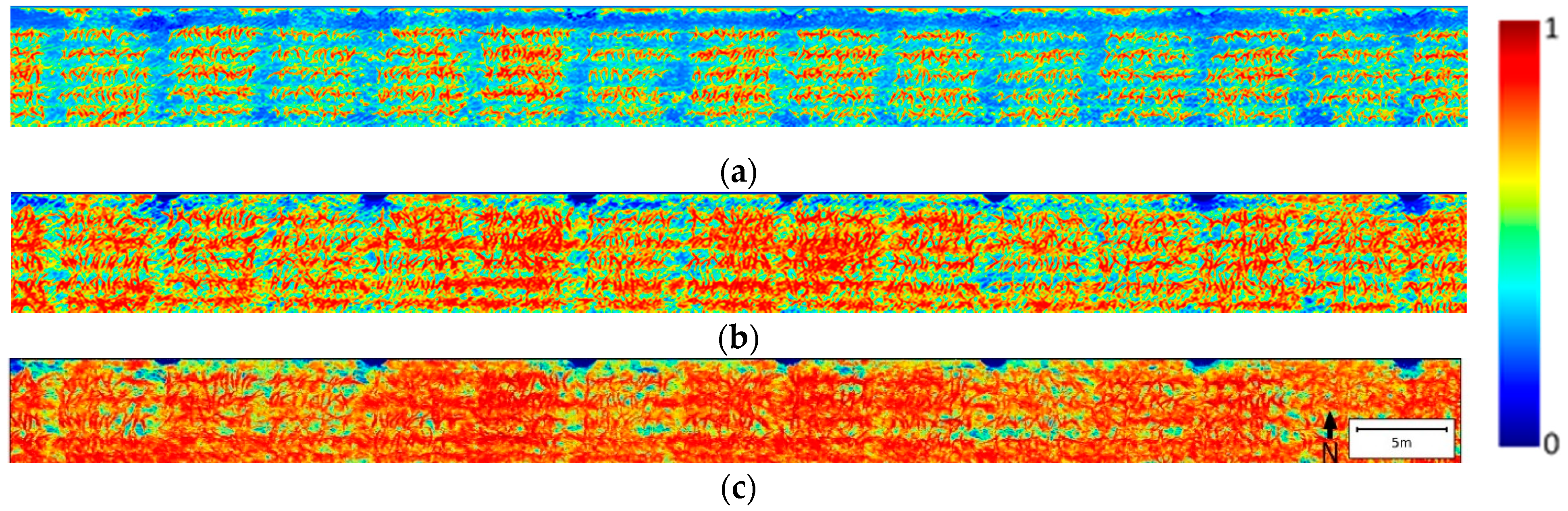
Figure 2.
The NDVI heatmaps for the whole field at three leaf stages with different accumulated after days planting (DAP). (a). 31 DAP, leaf stage V4; (b). 38 DAP, leaf stage V6; (c). 49 DAP, leaf stage V9.
Figure 2.
The NDVI heatmaps for the whole field at three leaf stages with different accumulated after days planting (DAP). (a). 31 DAP, leaf stage V4; (b). 38 DAP, leaf stage V6; (c). 49 DAP, leaf stage V9.

Figure 3.
The growth of corn plants in the Purdue ACRE field during the experiment at different DAPs.
Figure 3.
The growth of corn plants in the Purdue ACRE field during the experiment at different DAPs.

Figure 4.
The Relative Water Content (RWC) prediction model based on Partial Least Square Regression Relative (PLSR): measurement vs. prediction.
Figure 4.
The Relative Water Content (RWC) prediction model based on Partial Least Square Regression Relative (PLSR): measurement vs. prediction.

Figure 5.
(a) The NDVI of HN and Genotype B73 × Mo17 plot from V4 stage to the R1 stage (Obtained from the hyperspectral images); (b) The NDVI measurements across Day 1 (black dots). The red curve is the predicted NDVI diurnal variance by PROSAIL model. Parameters for the PROSAIL model for the corn canopies followed the work of Ishihara et al. in 2015.

Figure 6.
The mean RDR curves of six plant plots versus time (H). (a) HN and B73 × Mo17; (b) HN and P1105AM; (c) MN and B73 × Mo17; (d) MN and P1105AM; (e) LN and B73 × Mo17; (f) LN and P1105AM.
Figure 6.
The mean RDR curves of six plant plots versus time (H). (a) HN and B73 × Mo17; (b) HN and P1105AM; (c) MN and B73 × Mo17; (d) MN and P1105AM; (e) LN and B73 × Mo17; (f) LN and P1105AM.

Figure 7.
The NDVI of HN and Genotype B73 × Mo17 plot from V4 stage to the R1 stage. The raw NDVI plot was decomposed into the day-to-day trend () and diurnal pattern (). The red boxes are the days with incomplete data measurements due to the extreme weather conditions, which are 36, 37, 58, 59 and 60 DAP.

Figure 8.
The diurnal changes of NDVI summarized from 31 days and six experimental plots. The x-axis is the diurnal time in a unit of hour. The y-axis is the diurnal NDVI changes. The black line is the mean diurnal NDVI adjustment value. The shaded area is the 95% confidence interval. The red line is the 1st order piecewise fitted result for the mean diurnal NDVI adjustment value.

Figure 9.
The intersections between the adjusted NDVI’s diurnal changes and three different thresholds for proper imaging windows. The x-axis is the diurnal time in a unit of hour. The y-axis is the adjusted NDVI’s diurnal changes when adjustment at solar noon to be 0.
Figure 9.
The intersections between the adjusted NDVI’s diurnal changes and three different thresholds for proper imaging windows. The x-axis is the diurnal time in a unit of hour. The y-axis is the adjusted NDVI’s diurnal changes when adjustment at solar noon to be 0.

Figure 10.
The mean diurnal patterns and fitted results of other plant phenotyping features including RWC, Red and NIR. (a) RWC, diurnal pattern; (b) RWC, fitted result; (c) Red, diurnal pattern; (d) Red, fitted result; (e) NIR, diurnal pattern; (f) NIR, fitted result.
Figure 10.
The mean diurnal patterns and fitted results of other plant phenotyping features including RWC, Red and NIR. (a) RWC, diurnal pattern; (b) RWC, fitted result; (c) Red, diurnal pattern; (d) Red, fitted result; (e) NIR, diurnal pattern; (f) NIR, fitted result.


Table 1.
Parameters for the hyperspectral imaging sensor.
| Parameters | MSV-101-W |
|---|---|
| Camera model | acA780–75 gm |
| Spectrograph | SpecIM V10H |
| Frame rate | 30 FPS |
| Exposure time | 6 ms |
| Spectral resolution | 1.22 nm |
| Ground sample distance (GSD) | 0.5 cm/pixel |
| Spectral range | 376–1044 nm |
Table 2.
Number of samples after the quality check for six plant plots.
| Plant Plots | Number of Samples after the Quality Check |
|---|---|
| HN and B73 × Mo17 | 5070 |
| MN and B73 × Mo17 | 5092 |
| LN and B73 × Mo17 | 5083 |
| HN and P1105AM | 5108 |
| MN and P1105AM | 5084 |
| LN and P1105AM | 5093 |
Table 3.
Statistical analysis of the NDVI at Day 1 for six plant plots.
| Plant Plots | Mean | Highest | Lowest | Max Error |
|---|---|---|---|---|
| HN and B73 × Mo17 | 0.756 | 0.808 | 0.698 | 15.71% |
| MN and B73 × Mo17 | 0.732 | 0.780 | 0.689 | 13.33% |
| LN and B73 × Mo17 | 0.686 | 0.741 | 0.645 | 14.95% |
| HN and P1105AM | 0.759 | 0.817 | 0.717 | 13.96% |
| MN and P1105AM | 0.738 | 0.797 | 0.689 | 15.68% |
| LN and P1105AM | 0.687 | 0.733 | 0.648 | 13.20% |
Table 4.
The DTW distance scores between NDVI’s RDR curves of the plant plots with different nitrogen treatments and genotypes.
Table 4.
The DTW distance scores between NDVI’s RDR curves of the plant plots with different nitrogen treatments and genotypes.
| Plant Plots | HN and B73 × Mo17 | HN and P1105AM | MN and B73 × Mo17 | MN and P1105AM | LN and B73 × Mo17 | LN and P1105AM |
|---|---|---|---|---|---|---|
| HN and B73 × Mo17 | 0.00 | 0.33 | 1.37 | 1.48 | 1.40 | 2.31 |
| HN and P1105AM | 0.33 | 0.00 | 2.67 | 2.95 | 2.59 | 3.75 |
| MN and B73 × Mo17 | 1.37 | 2.67 | 0.00 | 0.20 | 0.14 | 0.60 |
| MN and P1105AM | 1.48 | 2.95 | 0.20 | 0.00 | 0.30 | 0.82 |
| LN and B73 × Mo17 | 1.40 | 2.59 | 0.14 | 0.30 | 0.00 | 0.30 |
| LN and P1105AM | 2.31 | 3.75 | 0.60 | 0.82 | 0.30 | 0.00 |
Table 5.
The DTW distance scores between NDVI’s RDR curves of the plant plots with different plant stages.
Table 5.
The DTW distance scores between NDVI’s RDR curves of the plant plots with different plant stages.
| Plant Plots | Distance Score between Early Stage and Late Stage |
|---|---|
| HN and B73 × Mo17 | 0.90 |
| MN and B73 × Mo17 | 1.26 |
| LN and B73 × Mo17 | 1.15 |
| HN and P1105AM | 0.25 |
| MN and P1105AM | 0.74 |
| LN and P1105AM | 0.63 |
Note: Early stage contains the first 15 days, and late stage contains the later 16 days.
Table 6.
Fit and error of the piecewise NDVI diurnal changing pattern model (Equation (8)) on assorted experiment plots.
Table 6.
Fit and error of the piecewise NDVI diurnal changing pattern model (Equation (8)) on assorted experiment plots.
| Plant Plots | R2 | RMSE |
|---|---|---|
| HN and B73 × Mo17 | 0.77 | 0.0058 |
| MN and B73 × Mo17 | 0.96 | 0.0036 |
| LN and B73 × Mo17 | 0.95 | 0.0032 |
| HN and P1105AM | 0.91 | 0.0038 |
| MN and P1105AM | 0.94 | 0.0034 |
| LN and P1105AM | 0.98 | 0.0022 |
Table 7.
Proper imaging windows for different thresholds of the NDVI changes caused by diurnal factors (when solar noon is the standard imaging time).
Table 7.
Proper imaging windows for different thresholds of the NDVI changes caused by diurnal factors (when solar noon is the standard imaging time).
| Thresholds | Suggested Imaging Time | Range |
|---|---|---|
| 0.01 | 12:45–14:40 | 1 h 55 min |
| 0.02 | 11:55–15:45 | 3 h 50 min |
| 0.03 | 10:55–16:30 | 5 h 35 min |
Table 8.
The fitted results of other plant phenotyping features.
| Features | R2 | RMSE |
|---|---|---|
| RWC | 0.97 | 0.16 |
| Red | 0.91 | 0.00094 |
| NIR | 0.98 | 0.0071 |
Publisher’s Note: MDPI stays neutral with regard to jurisdictional claims in published maps and institutional affiliations. |
© 2021 by the authors. Licensee MDPI, Basel, Switzerland. This article is an open access article distributed under the terms and conditions of the Creative Commons Attribution (CC BY) license (https://creativecommons.org/licenses/by/4.0/).
Share and Cite
MDPI and ACS Style
Ma, D.; Rehman, T.U.; Zhang, L.; Maki, H.; Tuinstra, M.R.; Jin, J. Modeling of Diurnal Changing Patterns in Airborne Crop Remote Sensing Images. Remote Sens. 2021, 13, 1719. https://doi.org/10.3390/rs13091719
AMA Style
Ma D, Rehman TU, Zhang L, Maki H, Tuinstra MR, Jin J. Modeling of Diurnal Changing Patterns in Airborne Crop Remote Sensing Images. Remote Sensing. 2021; 13(9):1719. https://doi.org/10.3390/rs13091719
Chicago/Turabian StyleMa, Dongdong, Tanzeel U. Rehman, Libo Zhang, Hideki Maki, Mitchell R. Tuinstra, and Jian Jin. 2021. "Modeling of Diurnal Changing Patterns in Airborne Crop Remote Sensing Images" Remote Sensing 13, no. 9: 1719. https://doi.org/10.3390/rs13091719
Note that from the first issue of 2016, this journal uses article numbers instead of page numbers. See further details here.